Innovation and Kondratieff II

Innovation is the true key to a more prosperous world!
   

Kondratieff

In a longer time perspective, western world economy appears to show a sort of returning waves of prosperous economic upswings and deleterious economic down turns. This effect is discovered and described by amongst others Kondratieff [1]. He coupled the economic upswings to major innovation breakthroughs. During the upswing however, somehow the innovative power seems to diminish and only to return in its full potential in the bottom, the winter of the cycle, to start the following cycle.

In the figure below a schematic draft of the last four cycles is presented [5].

 

First K-wave

The first Kondratieff wave is indicated to be coupled to the rise in steam engines and cotton industry. Well if we plot the number of steam engines used in the USA in a graph with the Kondratieff waves according to the wave patern as suggested by I. Gordon [9], the following image is obtained:

Quite astonishing, the growth in number of steam engines in the USA reached its maximum around 1910, in the middle of the spring of the third Kondratieff wave. The first steam engine was installed around 1776, well before the first kondratieff wave ended. The true rapid growth of steam power emerged beyond 1870, when the second Kondratieff wave was already in its winter period. The extreme and sudden decline of the steam engine from about 1909 was due only to the development of superior alternatives such as the internal combustion engine and the electrical engine. This decline, was a virtual collaps of an entire industry. 

The collapse came, while the steam engine industry was still in its increasing growth phase and was sudden and severe. Would there have not been any better alternatives the steam engine may have reached saturation around at the earliest in the 1990ies, as is shown in the following image:   

In this figure an S-curve is fitted, with the inflexion point set on 1909, around the year the highest number of steam engines were counted in the USA. Most of these numbers are obtained from old sensus data and are far from being exact. The effects of change of industry are however thus severe, that the inaccuracy in the data is of subordinate nature. 

What is striking is that the time span of the fitted S-curve from start to saturation easily stretches over all the Kondratieff waves now known to us. 

Second K-wave

The second Kondratieff wave is indicated to be coupled to the rise of the railway and steel industry. If we plot the total railway mileage in the USA a graph with the Kondratieff waves, the following image emerges:

Although allegedly responsible for the second wave, the greatest expansion of the USA railroad network started around 1880 and occurred only in the winter of the second wave. Furthermore the development of the railroad mileage and the number of steam engines initially developed almost parallel. Like the steam engine, the development of the railroad was strongly impaired by better alternatives, being the internal combustion engine powered road and air transport.  

If an S-curve is fitted on the development of the total milage in the USA, with an inflexion point set at 1895 again the time scale of full the diffusion of the rail roads untill its assumed saturation took from approximately 1830 until aproximately 1950, provided the better alternatives would not have been developed . So the total time span of the diffusion of railroads in the USA is about 120 years, spanning at least two Kondratieff waves.  

Third K-wave

The third Kondratieff wave is indicated to be coupled to the rise in the electrical industry and chemistry. If we plot the USA electrical power generation in the Kondratieff wave pattern, the following image can be derived:

Electricity production appears to coincide more with the fourth wave than the third K-wave. Although the first electricity distribution took place in 1882, installed in a power station built by Edison, the biggest growth of electricity production took place in the 1940-70ies. So this technology is more likely to have generated if any the upswing of the fourth Kondratieff wave instead of the third.

If an S-curve is fitted on the electricity production data, the graph below can be generated. From this graph, it appears that electricity is not yet fully diffused throughout the USA. The inflexion point of the fitted S-curve is set to 1988. 

Here again the time span between the first production in 1882 and saturation, estimated to be around 2040, is about 168 years, easily spanning over three K-waves. Remarkably, from 2008 the electricity consumption appears to stabilise or even to shrink.  It appears that yet a better alternative is about to break through and radically change the game. One of the most likely alternatives is solar power [10].


Fourth K-wave

The fourth Kondratieff wave is indicated to be coupled to the upcoming of automobiles. If we plot the number of licenced motorvehicles in the USA in the Kondratieff waves, the following image emerses:

ALthough the very first cars were built in the USA around 1895, in the end of the winter of the second K-wave, the biggest growth of the car industry did coincide with the spring and summer of the fourth Kondratieff wave.  

If an S-curve is fitted on the development of the number of cars, the inflexion point appear to be around 1980. The diffusion of cars throughout the USA is beyond its maximum growth, a full saturation will be reached around 2050.  

Here again the time scale of the diffusion of the technology of internal combustion engine driven road transport only diffuses at a pace slower than the kondratieff waves, it appears to take about 155 years up to full saturation. 



Concluding, undeniably, there are certain upswings and downturns in economy. These are however not so strongly coupled to the upcoming and downturn of innovative technologies as is often believed. The rate of diffusion of most (past) innovative technologies is of a different time scale than that of the Kondratieff cycles. The diffusion of steam engines in the USA up to the full potential is about 133 years, spanning almost three Kondratieff waves, the diffusion of railroads from its introduction in the USA in 1830 to its maximum capacity in 1930 is still 100 years, spanning two Kondratieff waves. The diffusion of road vehicles is from introduction around 1895 until its maximum, which is assumed to be 2050 is 155 years, again almost spanning three Kondratieff waves. Finally, the diffusion of electrical energy is from its start in 1882 till its maximum, likely reached in 2040 a full 168 years. Also spanning at least three Kondratieff waves.

To my opinion, not the innovation itself is the trigger for any economic upswing or downturn, but the valuation of the innovation and with that, the amount of money spend on a certain innovations by investors. Since any innovation appears to follow an S-curve (as long as no better alternative technology shows up), the early projections  of investors are by nature too negative.  Once the inflexion point is passed, the projections of investors are by nature too positive.

A first very illustrative and recent example of this effect is shown by the investors valuation of Facebook during its IPO. At the time of the public offering, the development of the number of subscribers to Facebook was already past its inflexion point. Linear extrapollation thus showed a far too bright future, and indeed investors were heavily overpaying [11].

Another illustrative example is the heavily underestimated development of the installed photovoltaic cell power production capacity. This because this development at the moment is still several years ahead of its inflexion point. The following figure represents the actually installed PV peak power, together with an S-curve fit and the 2011 and 2012 projections of the IEA, the leading energy research institute:

Facebook investors and highly recognized institutes with seasoned professionals seem to use linear extrapolations to estimate future development of innovations. To my opinion it is this behavior that drives the vast upswings and downturns in economy, not the underlying innovative technology.

Final remarks: The data collected all originate form various USA data sources. It is astonishing how well and how early in time the United States began to collect and publish all kinds of statistical information. Furthermore the USA was through most of the last two centuries the biggest economy on the planet. So not only is the data available from astonishingly early on, it appears to be both accurate enough and numberwise representative enough to sufficiently reflect global economic upswings and downturns of technologies.  

The S-curve fitting of innovation diffusion originates from relative early work of P.F. Verhulst stemming from as early as 1839 when he was describing population growth [12].


literature and sources

[1] Essay A. Spits (2002),  http://libertarian.nl/wp/2002/09/de-kondratiev-cyclus/

[2] Essay A. Spits (2008) http://libertarian.nl/wp/2008/12/kondratiev-winter/

[3] Interview D. van den Brink, J. kooistra (06-01-2012)
      http://managementscope.nl/magazine/artikel/617-dolf-van-den-brink-kondratieff

[4] http://de.wikipedia.org/wiki/Kondratjew-Zyklus

[5] http://nl.wikipedia.org/wiki/Kondratieff-golf

[6] http://faculty.washington.edu/modelski/IPEKWAVE.html

[7] Article by M.N. Rothbart  http://www.lewrockwell.com/rothbard/rothbard44.html


[8]  D. Lounsbury, Kondratiev Wave Theory Deflation and the Greater Depression http://www.deflationeconomy.com/kondratiev-wave.html

[9] The long wave analyst http://www.longwavegroup.com/principle/fourth_kondratieff_winter/fourth_kondratieff_winter.php 

[10] http://octrooifabriek.blogspot.nl/2012/05/we-will-innovate-our-way-out-of_24.html

[11] http://octrooifabriek.blogspot.nl/2013/01/betting-on-solar-power.html

[12] P.F. Verhulst,  “Notice sur la loi que la population poursuit dans son accroissement,”Correspondance mathématique et physique, 10, 1838 pp. 113-121,  http://books.google.nl/books?id=8GsEAAAAYAAJ&printsec=frontcover&hl=nl&source=gbs_ge_summary_r&cad=0#v=onepage&q=notice%20&f=false 

Innovation and kondratieff waves

Innovation is the true key to a more prosperous world. It is believed that global economic waves are virtually induced by innovations in a kind of cyclical motion.    

Kondratieff

In a longer time perspective, western world economy appears to show a sort of returning waves of prosperous economic upswings and deleterious economic down turns. This effect is discovered and described by amongst others Kondratieff [1]. He coupled the economic upswings to major innovation breakthroughs. During the upswing however, somehow the innovative power seems to diminish and only to return in its full potential in the bottom, the winter of the cycle, to start the following cycle.

In the figure below a schematic draft of the last four cycles is presented [5].

  

The Kondratieff wave appears to show four seasons: the spring, representing improvement, built up and construction; the summer: representing prosperity and consolidation; the autumn: representing a recession, the occurrence of a plateau or stabilisation phase and the winter representing a depression, a crisis, wherein severe liquidations occur.

Somehow it appears that we find ourselves in the winter of a Kondratieff cycle, which started according to most internet sources in 2000 with the burst of the internet bubble [1,2,3,4]. Some believe it may last until 2020, so some seven more years to come. Older articles predicted that the Kondratieff wave was to reach its winters end at around 2000. Others are more sceptical about the predictive power of the Kondratieff waves and its frequency. According to Rothbarth, the real business cycle is in no sense periodic, but is a continuing, wave-like motion that varies considerably in length and intensity.[7].

The question is, is this model of Kondratieff so sound? Well for the sake of fun, lets dig in some statistical history.

Alcohol consumption in the Netherlands

The first, very interesting and relative reliable historical statistical data over the timespan of most of the Kondratieff waves are figures on the per capita alcohol consumption in the Netherlands. The alcohol consumption is given by the following figure [8,9]:

Clearly a wave pattern can be distinguished. A first major dip in the consumption of alcohol can be seen around the year 1859, a second major dip in the per head consumption can be seen around approximately 1943. With some imagination, we can see three major peaks in the alcohol consumption, the first being around the year 1832, the second around the year 1890, the last, with more uncertainty since the peak, if any, is still in the making, around 1992. Here the peak and dip years are the ball park estimated mid points of the wave maxima and minima respectively.

From the deep and lasting dip around the 30ies and 40ies, it may be assumed that the alcohol consumption and the economy show a positive correlation. This means on average, with economic upswings, alcohol consumptie increases, with downturns the consumption decreases.

In the later Kondratieff models, for example as depicted below, the year 2000 appears to be the demarcation between autumn and winter. We appear to be somewhere half way wintertime and the true depression is only about to commence. This later Kondratieff model is constructed by I. Gordon of the longwave group, a Canadian financial research institution [12].

If we apply the later model to the alcohol consumption figures, the following combined image can be obtained. The datapoints in the blue field are taken as the exact seasonal turning points in the red wave model line:

Here only the last kondratieff wave seems to coincide with the Dutch alcohol consumption pretty well. With a little fantasy, the first wave somehow coincides somewhat with the consumption figures, though the second and third wave are not representing the historically collected statistical consumption figures.

Apparently, the predictive power of the kondratieff wave for alcohol consumption in the Netherlands is rather poor... 

(Un)employment in the Netherlands

Another very well documented figure is found in the unemployment statistics of the Netherlands. These figures are very likely to be directly coupled to the economic situation in the Netherlands. Since unemployment is supposedly inversely correlated to the economic upswing, the inverse of the unemployment is taken. This is the ratio between the total work force in the Netherlands and the number of unemployed people. This figure, a measurement for the employment varies between a number of about more than 120 and about less than 6 times as much people in the work force as the number of unemployed people. A high value of this indicator thus represents an economic high, whereas a low number represents an economic recession or even depression. These figures do show some wave like behaviour as well. If the Kondratieff low's and high's are inserted, the following combined figure can be obtained [11]:

Well, from this figure, it becomes clear that Kondratieff's model does not apply well to the Dutch (un)employment figures. It is likely, that in the Kondratieff spring and summer the employment should go up, in autumn and especially in winter employment would plummet. In the winter of the fourth wave (i.e. now), indeed employment is rapidly decreasing. For the rest, the Kondratieff  waves do not coincide well with the economic waves as represented by the employment figures.

Silver price in the Netherlands

Another figure to test the Kondratieff's theory is the -again very well documented- historical silver price development. In this figure, the silver price is expressed in guldens, a nowadays extinct currency, though over more than two centuries, the Euro represents only about eleven years. Thus, it makes more sense to recalculate the last eleven years to the gulden than to recalculate 200 years back in the history of the silver price to Euro. In the currency recalculation, a rate of exchange of 2,2 gulden per euro was used.

Since silver has actually been the material, our currency was made of until 1969 the long term development of the silver price was only due to debasement of the gulden, being a silver coin. Up to 1800 it contained 9,61 gram pure silver, from then until 1839 it contained 9,45 gram pure silver, from then until 1919 it contained 7,2 gram of silver, from then untill 1969 it contained only 4,68 gram of silver.  Hereafter, the silver price was decoupled from the gulden, being a mere nickel coin [14].

From the figure above, it can be concluded, that the silver price in the Netherlands does not coincide with the Kondratieff waves. Only the Kondratieff winter we are supposedly in at the moment, represents a strong increment in silver price.

Consequently, the three above statistically sound economic indicators from the Netherlands do not follow the Kondratieff waves at all. Is the Kondratieff theory wrong, well from these few statistical indicators, that conclusion appear to be too strong. The figures above do indicate however, that the Kondratieff model is not that sound as many do make believe....

[1] Essay A. Spits (2002),  http://libertarian.nl/wp/2002/09/de-kondratiev-cyclus/

[2] Essay A. Spits (2008) http://libertarian.nl/wp/2008/12/kondratiev-winter/

[3] Interview D. van den Brink, J. kooistra (06-01-2012)
      http://managementscope.nl/magazine/artikel/617-dolf-van-den-brink-kondratieff

[4] http://de.wikipedia.org/wiki/Kondratjew-Zyklus

[5] http://nl.wikipedia.org/wiki/Kondratieff-golf

[6] http://faculty.washington.edu/modelski/IPEKWAVE.html

[7] Article by M.N. Rothbart  http://www.lewrockwell.com/rothbard/rothbard44.html

[8] Tweehonderd jaar statistiek in tijdreeksen 1800–1999
      http://www.cbs.nl/NR/rdonlyres/7934A2DE-B87C-4CDF-8BC7-D34F02225620/0/200jaarstattijdreeksen.pdf

[9] Factsheet Alcoholconsumptie:
      http://stiva.nl/wp-content/uploads/downloads/2012/07/STIVA_factsheet-alcoholconsumptie_26jul121.pdf 

[10]  D. Lounsbury, Kondratiev Wave Theory Deflation and the Greater Depression http://www.deflationeconomy.com/kondratiev-wave.html

[11] Unemployment figures CBS:

http://statline.cbs.nl/StatWeb/publication/?VW=T&DM=SLNL&PA=71882ned&LA=NL

[12] The long wave analyst http://www.longwavegroup.com/principle/fourth_kondratieff_winter/fourth_kondratieff_winter.php 

[13] J. Luiten van Zanden e.a., The prices of the most important consumer goods, and indices of wages and the cost of living in the western part of the Netherlands, 1450-1800 http://www.iisg.nl/hpw/data.php#netherlands

[14] http://nl.wikipedia.org/wiki/Nederlandse_1_gulden

global number of motor vehicles

Innovation is the key to a more prosperous world!

As explained before, most growth of innovation can be mathematically captured by a relative straight forward growth curve. Mostly this growth curve can be properly modelled with an S-curve [1]. Let us now for the sake of fun have a look at the global development of the number of motor vehicles.  The numbers originate from a series of sources [4-12] and the fitted curve is a three parameter S-curve [2].

With fitting the S-curve, two quite bold assumptions were made:

The first assumption is that the final global car-saturation level is assumed to be equal to the 2010 car-penetration level of the USA. This level is about 808 cars per 1000 inhabitants [6].

The second assumptions is that in 2050, the global population is assumed to reach and stabilize at 10 bilion [10 x 10^9] inhabitants.

These assumptions are leading to a global saturation level of about 8.08 billion motor vehicles.

That the world is striving for a wealth comparable with that of the USA is astonishingly showed in the numerous presentations of Hans Rosling [3]. The assumption that in that line of wealth development, the world is striving to a similar penetration level of cars appears not to be too far fetched. Following these assumptions, the global number of motor vehicles will resemble the S-curve presented in the following figure:

In this figure, besides the statistical data available from numerous sources [4-12], two forecasts are given as well. The 2030 forecast in this figure originates from Dargay e.a. [5] and corresponds pretty well with the fitted S-curve. The 2050 forecast in this figure originates from the 2011 OECD international transport forum [4] and appears to be on the conservative side, when compared to the S-curve forecast.

From the assumptions made, we are going to have about eight times as much motor vehicles on the planet as we have now.

Further the number of vehicles on the planet is still growing ever faster, until about 2050, where the fitted curve changes from concave to convex.

Interestingly, these cars are in the future likely not to be all fossil fuel powered, because in fossil fuel production we are about to reach peak production. In the following figure is the yearly produced mineral oil is presented. It can be seen that the production is, though still increasing, is in its convex phase, past its inflexion point [16]. The data from 2012 and 2013 are the forecasts given by the IAE [17]. With a slowing growth of mineral oil production and an increasing growth of the number of vehicles, soon there is simply not enough mineral oil to feed all these vehicles.

So here there is ample space for innovation! More efficient vehicles and alternative energy sources, I cant wait to see them coming!



[1] http://www.slideshare.net/HendrikdeLange/s-curve-presentation-wwwcrowdfundersnl 

[2] The Rise and Fall of Infrastructures, A. Grübler (1990) http://www.iiasa.ac.at/Admin/PUB/Documents/XB-90-704.pdf

[3] http://www.ted.com/talks/view/lang/en//id/1101

[4] http://www.huffingtonpost.ca/2011/08/23/car-population_n_934291.html

[5] http://www.xesc.cat/pashmina/attachments/Imp_Vehicles_per_capita_2030.pdf

[6] http://en.wikipedia.org/wiki/List_of_countries_by_vehicles_per_capita

[7]  http://oica.net/category/production-statistics/

[8]  http://www.nationmaster.com/graph/tra_mot_veh_pro-transportation-motor-vehicle-production&date=2000-01-01

[9]  http://hypertextbook.com/facts/2001/MarinaStasenko.shtml

[10]  http://www.huffingtonpost.ca/2011/08/23/car-population_n_934291.html

[11]  http://www.worldometers.info/cars/

[12]  http://www.car-history.org/the_begining_of_19th_century_in_car_history/

[13]  http://people.hofstra.edu/geotrans/eng/ch6en/conc6en/ch6c1en.html

[14]  http://cta.ornl.gov/data/tedb30/Edition30_Full_Doc.pdf

[15] Analysis  of   Logistic  Growth  Models, A.Tsoularis, Res. Lett. Inf. Math. Sci,  (2001) 2,  23-46

[16] http://www.bp.com/sectionbodycopy.do?categoryId=7500&contentId=7068481

[17] http://www.iea.org/Textbase/npsum/weo2012sum.pdf 

huizenprijsontwikkeling

Wie de toekomst wil lezen moet in het verleden bladeren...

Uit het dagblad "de Tijd" 1-1-1894:
De waarde der perceelen, waarop naar verhouding hypotheek werd verstrekt, hield men zoo lang mogelijk hoog, doch eindelijk moest de waarheid beslissen, de natuurlijke waard werd weder besteed, en het tekort was: verlies. Alzoo ging het algemeen vermogen op tweederlei wijze terug, èn dat van den grondeigenaar èn dat van den hypotheekgever. Niemand kan dat weerhouden. Komen er tijden, dat de ondernemingsgeest weder levendiger wordt, dan zal 't tegenovergestelde van het tegenwoordige plaatsvinden, maar deskundigen, die deze geschiedenis met belangstelling medeleven, zullen steeds weten te onderscheiden wat de werkelijke waarde is en wat men besteedt.


Zal het nu anders zijn? Nee, maar er gloort licht aan de horizon!

Met weinig fantasie is er een griezelige gelijkenis te herkennen in een algemene theorie die bubbles beschrijft en de historische ontwikkeling van de gemiddelde huizenprijs in Nederland. Deze theorie kan worden weergegeven met een algemeen diagram. Dit diagram en de onderliggende theorie is in 2008 opgesteld door J.-P. Rodrigue [1]:

Een bubble-scenario vertoont volgens deze theorie een stille fase, een bewustwordingsfase met een "bear trap", een manie-fase met een absolute top en een leegloop-fase met een "bull trap". 

De ontwikkeling van de gemiddelde huizenprijs wordt weergegeven door [2,3,4]:

In dit diagram zijn een bewustwordingsfase met een "bear trap" in het begin van de jaren 80 te herkennen. Vervolgens is een manie-fase te onderscheiden met een top in 2007, en vervolgens een leegloop-fase met een "bull trap" in 2009. 

Zou het scenario van Rodrigue op de huizenprijs worden toegepast, dan zou het toekomstbeeld er ongeveer als volgt kunnen uitzien: 

Een terugval van de gemiddelde huizenprijs tot circa 30 000 euro, waarbij de gemiddelde huizenprijs met ruim 80% daalt. Het dieptepunt ligt in dat geval ergens voorbij het jaar 2020. 

Is dat een reële inschatting, een daling van ruim 80%? Als de huizenprijsontwikkeling in de jaren 20 tot medio jaren 40 in detail wordt weergegeven, ontstaat het volgende beeld [4]: 

Er vond van 1930 tot 1936 een afname van de gemiddelde huizenprijs plaats van meer dan 10 k€ tot 2 k€, ofwel een daling van 80%. pas in 1944 kwam de prijs weer op het niveau van de top van 1930. Met andere woorden, een daling van de gemiddelde huizenprijs van 80% is mogelijk, sterker nog een dergelijke daling heeft zich in de twintigste eeuw al eens voorgedaan. 

In de aanloop naar de piek in 1930 was er weliswaar sprake geweest van een gestegen huizenprijs, maar deze bedroeg slechts rond de 50% ten opzichte van de gemiddelde prijs tussen 1922 en 1928. Dit lijkt in geen geval een bubble, zoals Rodrigue hem beschrijft. Tot 2007 heeft zich daarentegen een onafgebroken stijging van de huizenprijs voorgedaan van gemiddeld 60 k€ in 1983 tot gemiddeld 250 k€ in 2007, ofwel een stijging van ruim 300%. De recente stijging is, in relatieve zin, dus zes keer zo groot als de stijging aan de vooravond van de laatste grote depressie uit de jaren 30.

Is er iets aan te doen om dit scenario af te wenden? 

Ja, door grof geschut in te zetten. Dit kan door drastische belastingverlagingen, wettelijke verlaging van de hypotheekrente tot bijvoorbeeld Euribor of een drastische verruiming van de hypotheekrente-aftrek. Ook een verdere verruiming van de maximum toelaatbare schuld van de koper zou een mogelijkheid kunnen zijn. Verder zouden centrale banken hypotheekportefeuilles van banken kunnen opkopen. Al deze maatregelen hebben een inflatoir karakter en geven weliswaar een uitstel van de leegloop-fase, maar ook een sterke vergroting van de (staats)schuld. Juist een ongeremde verruiming van de (hypotheek)schulden heeft deze bubble veroorzaakt. Het vergroten van de schuld zal dus het probleem slechts tijdelijk opschorten, zeker niet oplossen, eerder nog versterken.  

Thans heeft ons landelijk bestuur om begrijpelijke redenen een andere weg gekozen:

De hypotheekrenteaftrek wordt beperkt en er wordt voor deze aftrek een aflossing binnen 30 jaar vereist. Daarnaast wordt de belastingdruk alleen maar verhoogd en lijken de salarissen te gaan dalen. Ook wordt de financieringsruimte verlaagd naar maximaal 4 maal het brutto jaarsalaris, terwijl eerder tot 6,5 maal het brutto jaarsalaris kon worden gefinancierd. Als laatste zal de financiering van 106% van de verkoopprijs verder worden verkrapt tot onder de 100%. Dit alles verlaagt de financieringsruimte van de koper en heeft een deflatoir karakter. 

Een bijkomend effect, wat deze ontwikkeling nog versterkt is een oplopende werkloosheid. Ook deze stijging heeft een negatief effect op de koopkracht van de Nederlander en verkleind de collectieve financieringsruimte. 

Er blijkt een sterke correlatie te bestaan tussen een dalende huizenprijs en een oplopende werkloosheid. Deze twee effecten lijken elkaar wederzijds te versterken. Tussen 1930 en 1933 daalde de huizenprijs met 60% en steeg de werkloosheid van 4,9% naar 16,9%; meer dan een factor 3. Tussen 1978 en 1982 daalde de huizenprijs met 40% en steeg de werkloosheid van 4,6% naar 10,7%; meer dan een factor twee. Beide stijgingen van de werkloosheid zijn daarnaast de twee sterkste stijgingen in de laatste 200 jaar [5].

Een daling van de huizenprijs van 80% zoals in het bubble-scenario van Rodrigue zou dus gepaard kunnen gaan met een stijging van de werkloosheid met een factor vier. Dit betekent dat het werkloosheidspercentage tot 25% zou kunnen stijgen. Een regelrechte ramp, die in Spanje en Griekenland al werkelijkheid is geworden.

Een ander aspect dat effect op de huizenprijs heeft is de bevolkingsgroei en de daarmee samenhangende toenemende vraag. Ons gevoel zegt dat de prijs wordt gevormd door vraag en aanbod... Voor de prijs van huizen lijkt dit echter niet het geval. De prijs wordt hier thans veeleer gevormd door de financieringsruimte van de koper enerzijds en de bereidheid van de verkoper om verlies te nemen anderzijds.  De financieringsruimte van de koper is al aan het afnemen, de bereidheid van de verkoper om verlies te nemen zal met de tijd gaan stijgen. De groei van de bevolking in Nederland zit bovendien niet in een groeiende hoeveelheid starters, maar in een groeiende hoeveelheid senioren [6]. 

Dat een sterke vraag alleen is niet genoeg is voor een stijging van de huizenprijs, blijkt voorts uit de wegblijvende grote stijging van de huizenprijs aan het eind van de jaren 40 en gedurende de jaren 50.  Er heerste een knellende woningnood, met een veel grotere vraag en een veel geringer aanbod dan nu. Toch gingen toen de prijzen gingen niet door het dak. Er was destijds voor kopers onvoldoende financiering te krijgen.  

Met andere woorden het zoet van de lichtzinnig vergrote financieringsruimte en toegang tot makkelijke kredieten van de periode tussen 1980 en 2010 en de daarmee gepaard gaande inflatie maakt plaats voor het zuur van een krimpende financieringsruimte en de daarmee gepaard gaande deflatie. Het gevolg is dalende huizenprijzen, toenemende restschulden,  oplopende werkloosheid en versterkte persoonlijke gevoelens van falen, mislukken en depressiviteit. Deze laatste gevoelens worden door Rodrigue passend gevangen in de termen "fear", "capitulation" en "dispair". 

In mijn ogen is dit alles de verwijtbare schuld van een generatie politici en bankiers die in de jaren 80 het roer overnam van een generatie die nog echt schrale tijden had gekend. De solvabiliteit van banken werd verkleind, de kredietkranen werden opengedraaid. Alsof ons collectieve geheugen niet verder reikt dan ongeveer 60 jaar, zien wij ons hierdoor overeenkomstig onze grootouders thans opnieuw met een drastische crisis geconfronteerd. Een crisis die zich nog aan het ontvouwen is en waarop nauwelijks een mens een antwoord lijkt te hebben. 

Dit alles terwijl al in 1894 de oplossing lijkt te zijn aangereikt: verlies nemen en ondernemingsgeest tonen. 

In dat licht bezien, is innovatie het juiste antwoord op een dreigende depressie. Innovatie in plaats van inflatie, innovatie in plaats van deflatie. De wereld heeft het geluk dat er een hele grote innovatiegolf in razend tempo op ons af komt. Deze innovatiegolf is er één van een complete omwenteling van fossiele energieopwekking naar fotovoltaïsche energieopwekking [7,8,9]. 

Daadkrachtige leiders tonen lef door niet langer geld te pompen in het overnemen van kredieten van banken. Daadkrachtige leiders tonen lef door niet langer de huizenkoper zijn financieringsruimte af te pakken. Daadkrachtige leiders tonen lef door massaal in te zetten op het investeren in nieuwe energieopwekking en overige innovatieve technologie. Hiervoor is een ondernemingsgeest nodig. Een verdere welvaartssprong die ondernemingsgeest van onze leiders vraagt, is die van het uitbannen van het Europese verbod op het genetisch ontwerpen van hoogproductieve voedselgewassen. Beide innovatieve technologieën genereren nieuwe banen en creëren daarmee welvaart. Beide technologieën hebben bovendien een positief effect op het milieu en verkleinen de uitstoot van broeikasgassen. Deze technologieën vervullen bovendien de belangrijkste basisbehoeftes van de mens: energie en eten. 

Leiders van Europa, toont ondernemingsgeest!  

Bronnen en literatuur

[1]  J.P. Rodrigue, http://canadianfinanceblog.com/is-the-current-market-a-return-to-normal/

[2] Gegevens van het CBS huizenprijs (teruggerekend uit geïndexeerde gegevens)

http://statline.cbs.nl/StatWeb/publication/?VW=T&DM=SLNL&PA=71533NED&D1=0-1,3-4&D2=0-1,6&D3=0&D4=16,101,186,203,220,237,254-257,259-261,263-265,267-269,271-274,276-l,!297&HD=110728-0930&HDR=G1,T&STB=G2,G3

[3] Gegevens van de NVM huizenprijs

http://www.nvm.nl/wonen/marktinformatie/historische_woningmarktcijfers.aspx

[4] Deze gemiddelden zijn gegenereerd aan de hand van veilinggegevens en advertenties uit edities van de volgende kranten in de jaren 1922-1944: de Tijd, het Algemeen Handelsblad, de Nieuw Rotterdamse Courant, het Nieuws van den Dag en de Standaard. De jaarlijks gemiddelde prijzen hebben als basis telkens ten minste 50 individuele gegevens. Van de jaren 1945 en 1946 zijn niet genoeg gegevens gevonden om een robuust gemiddelde te genereren. Deze kranten zijn digitaal beschikbaar via de Koninklijke Bibliotheek: http://kranten.kb.nl/

[5] gegevens CBS werkloosheid: 

http://statline.cbs.nl/StatWeb/publication/?VW=T&DM=SLNL&PA=71882ned&LA=NL

[6] gegevens CBS bevolkingsopbouw: 

http://www.cbs.nl/nl-NL/menu/themas/bevolking/cijfers/extra/piramide-fx.htm

[7] blog: Betting on solar power? http://octrooifabriek.blogspot.nl/2013/01/betting-on-solar-power.html

[8] blog: Energy revolution! http://octrooifabriek.blogspot.nl/2012/11/energy-revolution.html

[9] blog: We will innovate our way out of recession

 http://octrooifabriek.blogspot.nl/2012/05/we-will-innovate-our-way-out-of_24.html

Betting on Solar power?

Yesterday the news caught my eye that Warren Buffet is investing in solar power. Actually most sources indicate he is "betting" on solar power rather than investing [4].

To my opinion, would he be betting he would have bought Facebook shares last summer!

Here is why:

At the time Facebook published its prospects on the IPO, the development of the number of users of Facebook was pretty much represented by the following graph. Honestly, the last point on the graph was not yet available, though matches pretty accurately with the model being a fitted S-curve.

Investing in Facebook at the IPO means investing in a company that is in a phase where the growth diminishes and is closing in on saturation. So there is still growth, though not one justifying a market value representing a fivefold higher future profit than is generated at the moment. Deep respect for the Facebook team to have sold their company shares at such a good price!

Whereas Facebook as innovation is almost through the "late majority", Solar silicon PV cell power generation is in its "early adopter" stage, as can be seen from the following graphs [1]:

Here again an S-curve is fitted on the data available. The installed peak capacity at 2012 years end is about 200 GW,  around 2,5% of the total global electrical energy produced:

In this graph the S-curve is extrapolated beyond the point where peak capacity surpasses the electric power demand in around 2024.

Being the first does not really matters as long as the generated PV power more expensive than conventionally available power. Well here is the interesting part, these PV power prices have come down [2,3]:

In this graph, BOS indicates Balance of System, including wiring, switches, support racks, inverter, and batteries. The data represented in the above graph are up to 2000 based on BOS calculations, from 2000 onwards, they are calculated using LCOE, which indicates the Levelized Cost of Energy, in which capital investment write off is incorporated. 

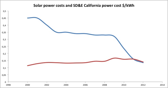
Since the late 50ties till 2011 the PV solar generated price of a kWh came down from about 250 dollar to about 13 dollarcents. Because this drop in price is so huge, the above presented graph lacks the scale to see in detail what is happening in the last few years. In the graph below, last twelve years are presented in more detail.

The blue line represents the price of solar generated power on average throughout the USA, the red line represents the average tarifs (domestic, small and large scale industrial) on power supplied by San Diego Gas and Electric (California), a commercial electric power supplier.

In 2011, solar power could -USA wide- be produced at the same price as commercially available electricity in California. In 2012 it appears that solar power prices even push down commercial prices, which means that traditional power generation in California is facing a serious, game changing competitor.

Just to complete the math, what did Mr. Buffet get for his approximate 2.5 billion dollars:

A 597 MW power plant under construction, being bought for about 4.18 $ per W. This is a considerable sum of money, invested in a plant at the antelope valley, about 90 km north of Los Angeles. Here, it is not a coincidence, insolation is at its highest throughout the USA [image from NLRE]:

If we assume this plant on average during a full 24 hours produces 40% of its peak capacity, it can turn over about 272 million dollars a year at an energy price of 13 cents per kWh. If maintenance and operation of the system is estimated to be 10% of the income, than a yearly income of about 250 million dollars seems reasonable, generating a 10% return on investment. Should the price of a kWh drop another 50% than a return on investment of about 5% could still be feasible.

It is very likely that Warren Buffet has studied similar material and came to the following or similar conclusions:

- Solar power in California can now be generated at the same price as commercially available electric energy, grid parity has become a fact.

- Investing in Solar PV generation plant means investing in the "early adopter stage" of a potentially booming new industry.

- Solar power is not dependent on price fluctuations in oil, gas, coal or uranium which all tend to go up in longer perspective [5].

- A California based solar power plant can return between 5% and 10% on investment.

- Besides economic factors, ecological factors, like carbon dioxide taxation could further provide reasons to go solar.



If investing in this early stage, yet profitable industry is seen as betting, than boy, do I wish our European politicians and European central bankers were betting more!






Literature/sources of data:

[1] http://www.bp.com/sectionbodycopy.do?categoryId=7500&contentId=7068481

[2] http://www.cpuc.ca.gov/PUC/energy/Electric+Rates/ENGRD/ratesNCharts_elect.htm

[3] http://www.bnef.com/WhitePapers/download/82


[4] http://www.huffingtonpost.com/2013/01/03/warren-buffett-solar-power_n_2398816.html


[5] http://octrooifabriek.blogspot.nl/2012/11/energy-revolution.html

Energy revolution

Innovation is the most powerful key to a more prosperous world. Innovation will drastically change the world. How drastically, well read and be surprised, the energy revolution has begun!

Over the last fifty years, we see a steadily increased consumption of oil, which may represent our global prosperity [1,2]. In these 50 years we see only three times a decline in yearly oil consumption:

In 1973, being the first oil crisis, resulting from the Yom Kippur war, lasting for two years.
In 1978 being the second oil crisis, resulting form the Persian revolution lasting four years.
In 2008 being the US banking crises, lasting two years.

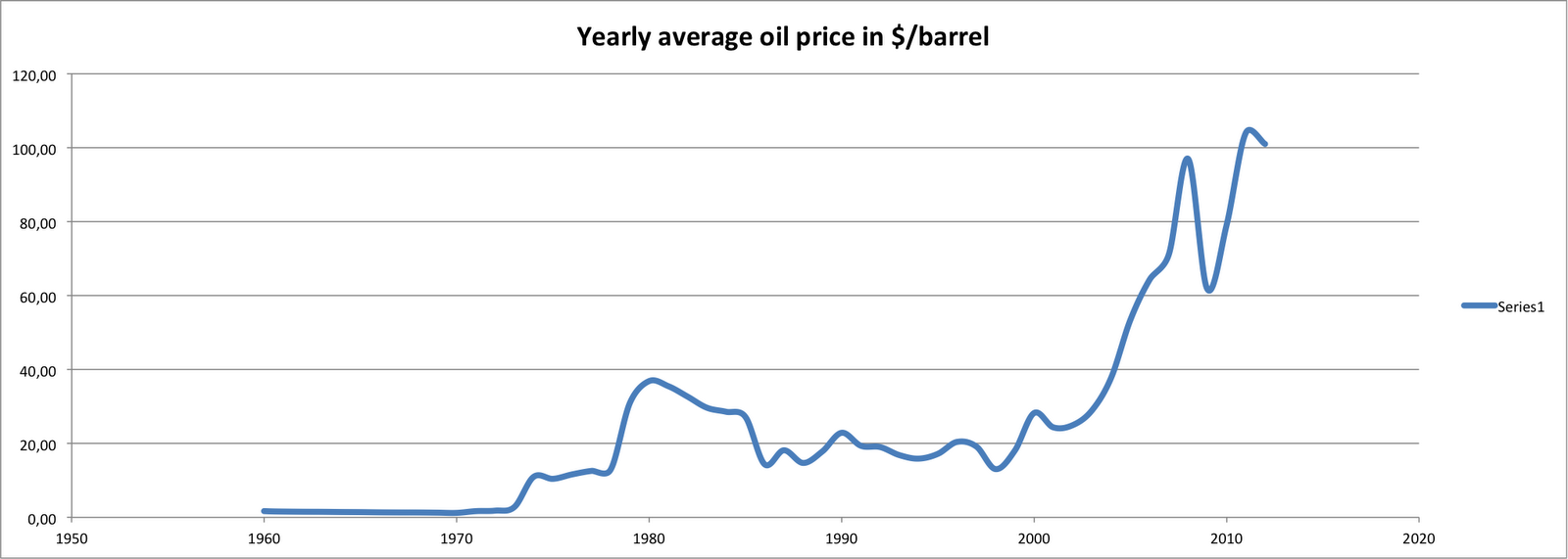
In the same timespan, the yearly average oil price has developed as [3]:

Also in this figure, the first and second oil crises can be seen, as is the 2008 US banking crisis. Further the price has fallen considerably after the 1986 crash, after the 1998 asian banking crisis and after the 2000 burst of the dot com bubble. Further we can see the extreme price surge from the 2003 US invasion in Iraq, and to a much less extend the invasion of Iraq in kuwait in 1990.

What is more fascinating, is that both price and consumption go up over time. The more we use, the more we pay.

We may think that for coal this price development is different, well it is not [3]:

Here again the big drop in coal price is seen following the US banking crisis.

To be complete, the natural gas prices show an image slightly different, though with similar implication [3]:

So all our fossil energy sources show at least a tenfold increase in price since the mid 70ties. This might arguably be the result of a heavily inflating dollar, well maybe not. Opposed to these price development, silicon poly-crystalline solar cell prices has almost constantly dropped. This development has evolved irrespective of any oil crisis and irrespective of any country invading another [4]:

Consequently: in the same time all fossil energy prices went up more than ten fold, PV cell prices went down a factor 100. Furthermore the trends are that fossil fuels will get more expensive, whereas Photovoltaic energy will get less expensive.


No wonder that the amount of installed (peak) capacity of PV power is exponentially rising [1]:

If the S-curve fit is expanded into the future, we will see that the installed peak PV capacity will reach and surpass our electrical energy consumption already in 2024 [1].

This is very good news! It means abundant and cheap energy. It means less incentives to start wars in the gulf region. It means far less carbon dioxide emissions. It means a much cleaner environment.

Thank you technology for making this possible! Thank you inventors of this technology. Thank you, silicon industry for ever producing more and better available silicon!!!

THANK YOU!!!!!



literature/sources:

[1] Statistical review of the world energy 2012, BP

 http://www.bp.com/sectionbodycopy.do?categoryId=7500&contentId=7068481

[2] IEA highlights October 2012

http://omrpublic.iea.org/currentissues/full.pdf

[3] World Bank pink sheets 2012, world prices of commodities and indices, historical data

http://econ.worldbank.org/WBSITE/EXTERNAL/EXTDEC/EXTDECPROSPECTS/0,,contentMDK:21574907~menuPK:7859231~pagePK:64165401~piPK:64165026~theSitePK:476883,00.html

[4]  Re-considering the Economics of Photovoltaic Power, M. Bazilian e.a. (May 2012)

http://www.newenergyfinance.com/WhitePapers/view/82

Patent density

Driven by pure curiousity, I 've wondered what the patent density around the world would look like.

From datasets made available by gapminder [1], it is posible to calculate the number of patents in force per capita. For the top 45 countries the results are shown below, wherein the abscis is expressed in a logarithmic scale.

I thought, that the patent density would be an great indicator for e.g. prosperity of a nation.... well seen the astonishing 7 granted patents per capita in Gibraltar, more than 1000 times the patent density in Japan, this figure more reflects the size of the country than anything else.

What does this patent density tell us?  Well the amount of protected patents does not even reflect the amount of infringement cases. In Canada for instance, with about 10,4 active patent rights in force per 1000 inhabitants, less infringement cases are brought to court than in the USA with about 4,3 active patents per 1000 inhabitants. So this indicator is not indicative for infringement behaviour. 

Furthermore, the fact that Swasiland, with a relative low developed technology has a higher patent density than e.g. Switserland, Japan and the USA indicates that patent density isn't a great indicator for drawing any conclusions on prosperity or technology advancement levels of a country...

I can only conclude that patent density is a very lousy indicator. Too bad....

[1] http://www.gapminder.org/data/